Package com.openinventor.imageviz.engines.imagesegmentation.classification
- Spectral: each attribute is a channel pixel value from a color or multi-band image.
- Spatial: each attribute is measurement on a given neighborhood of the target pixel. Generally these measurements reveal the local texture surrounding the pixel.
Pixel classification methods can be split into two categories:
- Unsupervised classification: the input image is automatically partitioned into a predefined number of regions.
- Supervised classification: regions are learned thanks to a training step on representative samples.
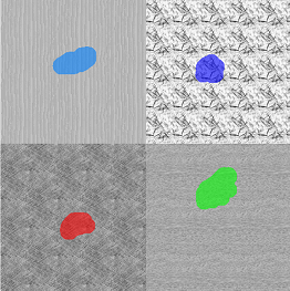
Texture supervised classification tools aim to perform an image segmentation based on local textural features when typical intensity based segmentation tools are not appropriate.
A texture classification workflow is composed of 3 steps:
- Creation of a texture classification model
- Learning of the texture model on representative training images
- Application of the texture model to a grayscale image (texture segmentation)
During the learning step, all the selected features are computed on a local neighborhood of pixels belonging to labels defined in a training image. A subset of discriminant features is retained and only these features are computed during the segmentation step.
 |  |  |
Two categories of textural feature descriptors are available:
- Features based on co-occurrence matrices.
- Features based on intensity statistics.
Co-occurrence based features
A co-occurrence matrix expresses the distribution of pairs of pixel values separated by a given offset vector over an image region.
From co-occurrence matrices one can derive statistics called Haralick's indicators that are commonly used for describing texture features
For more information about co-occurrence matrix and Haralick's textural features, please refer to the SoCooccurrenceQuantification2d engine documentation.
The term texton refers to a basic texture element whose size and shape can define a set of vectors used for determining co-occurrence matrix. A texton expresses orientation and spacing of a repeated texture pattern (e.g., stripes).
Data Ranges: The minimum and maximum values of the co-occurrence matrix are extracted from the data min max of the first image used during the learning step. Consequently, for enriching a classification model or segmenting several images with a same model, all images must have a data range consistent with the first training image. If not, the data must be normalized before processing
Two groups of co-occurrence based features are available. Basically the 13 Haralick's texture features are computed for each co-occurrence vector defined by the input texton. Then the features can be applied in two ways:
- Directional co-occurrences: each co-occurrence vector of Haralick's features is considered as a separate textural feature. Thus 13 Haralick's features times the number of co-occurrence vectors are computed.
- Rotation invariant co-occurrences: for each Haralick's feature, 3 statistics over all offset vectors are considered as separate textural features (range, mean and variance). Thus 39 texture features are computed.
Note that using directional features provides generally better result for anisotropic material (fibers) but the acquisition process must ensure a constant orientation. If not, a rotation should be applied as preprocessing to make the input image match with the training image orientation.
Intensity statistics based features
which are described in the Histogram category of the measurement list of individual analysis. Three groups of intensity based statistics are available:
- First order statistics: mean, variance, skewness, kurtosis and variation.
- Histogram statistics: histogram quantiles, a peak measurement, energy and entropy.
- Intensity: input image intensities.
The second group computes first a local histogram from which the features are extracted. The histogram minimum and maximum values are extracted from the data min max of the first image used during the learning step. All intensity statistics based features are rotation invariant. Consequently, the extracted value does not change when an arbitrary rotation is applied to the input image
The texture model creation step consists in initializing a classification object by defining:
- The number of classes to define, i.e., the maximum label of the training images.
- The textural feature groups to compute for classifying textures.
- The radius range of the local neighborhood for computing texture features.
The radius defines the disk or sphere window centered on a target pixel where the textural features are computed. This parameter has a strong influence on the segmentation result and leads to indeterminate areas at texture boundaries. The radius of analysis must be sufficiently large to model the whole texture. If the radius is too small, the algorithms will fail to classify complex textures. If the value if too large, the algorithm will create strong artifacts at region borders and will be computationally inefficient. Therefore a range of radius is evaluated by the training step in order to simplify the tuning of the algorithm. This range is defined by a minimum, a maximum and a step.
This step consists in enriching a classification model by learning on a gray level image that has been labeled. Each label value of the training image identifies a class. Consequently, a same label value can be used in different connected components.
Feature extraction
For each labeled pixel of the training image, the algorithm extracts all texture features belonging to the groups selected in the texture model. These newly extracted features increase the learning-set and enrich the model.
Training border management: Note that all pixels within the analysis radius of a labeled pixel will be considered for the feature extraction, even if they don't have the same label value than the considered pixel. It means that the number of pixels use for training is greater than the number of the labeled pixels.
Once the features are computed on the training image, the classification model is updated and all the features that are not enough discriminating or too much correlated with another feature are rejected.
For a given set of features, a separation power expressed in percent computed. This value quantifies how this set of features discriminates the learned classes. A measure is rejected if its contribution does not increase enough the separation power of the classification model.
The minSeparationPercentage parameter is a rate in percent that indicates the minimum relative increase of the separation power brought by a feature to select it. A higher value will tend to reduce the number of features actually used for classification and thus to lower the computation time of the classification.
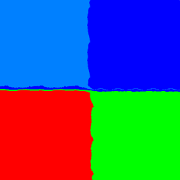
This step classifies all pixels of an image using a texture model and generates a new label image where a label corresponds to a texture class.
For all pixels of the input image, the algorithm extracts the texture features selected in the classification model and computes their Mahalanobis distance to each class center of the model.
Finally, the classification step outputs:
- a label image where each pixel value corresponds to the identifier of the closest class (i.e., its label intensity used at the training step).
- a float image where each pixel value corresponds to a metric representing an uncertainty score (uncertainty map). By default this metric is the distance to the closest class but it can be also a score taking into account the level of ambiguity of the classification or the distance to each learned class .
Combining the uncertainty map and the classified label image can be useful to reject mis-classified pixels and apply post-processing in order to improve the classification result.
-
Class Summary Class Description SoAutoIntensityClassificationProcessing SoAutoIntensityClassificationProcessingclassifies all pixels/voxels of an image using the k-means method.SoSupervisedTextureClassificationProcessing2d SoSupervisedTextureClassificationProcessing3d -
Enum Summary Enum Description SoSupervisedTextureClassificationProcessing2d.CoocTextonShapes This enum defines all type of measures used for texture classification.SoSupervisedTextureClassificationProcessing2d.FeatureGroups This enum defines all type of measures used for texture classification.SoSupervisedTextureClassificationProcessing2d.OutMapTypes SoSupervisedTextureClassificationProcessing3d.CoocTextonShapes This enum defines all type of measures used for texture classification.SoSupervisedTextureClassificationProcessing3d.FeatureGroups This enum defines all type of measures used for texture classification.SoSupervisedTextureClassificationProcessing3d.OutMapTypes