Package com.openinventor.imageviz.nodes.measures
Measurements allow to quantify dimensional, shape or intensity features from objects of the input data. For instance, a set of measurements has to be selected using SoLabelAnalysisQuantification, SoLabelFilteringAnalysisQuantification or SoGlobalAnalysisQuantification engines. Here are described general priciples that help to understand most of the ImageViz predefined measurements.
The SoDataMeasurePredefined class contains the list of the measurements that are immediately available in ImageViz. Each measurement is identified by a PredefinedMeasure enumerate. The name of these enumerates may end with 2D or 3D:
- 2D indicates that a mesure is only supported with 2D images,
- 3D indicates that a measure is only supported with 3D images,
- if this information is omitted, the measure works on both types of images.
Enumerates having a name starting with GRAY or INTENSITY are measurements based on the intensity image input.
These measures don't support intensity images with more than one channel. Please use the SoColorGetPlaneProcessing2d engine to extract the required channel before computing the intensity measurement.
Please see section Image Analysis to know how to perform analysis on such measurements.
Here are described some computations of global characteristics of a shape.
The first order moments define the centroid or center of mass.
In the continuous case they are defined as: 


and in the discrete case as: 


Where  is a point of the object X, g its gray level intensity and
  the area of X.
For gray level images  , for binary images just consider
  .
.
Note :
- Name of ImageViz measurements based on these computations start with GRAY_ if the moments are computed weighting the result by the graylevels of the intensity image (e.g., GRAY_BARYCENTERX).
- Other measurements don't take into account the graylevels of the intensity image (e.g., BARYCENTERX).
- If the intensity image given to the analysis engine is a binary image, both types of measurement will output the same result (GRAY_BARYCENTERX = BARYCENTERX).
Second order moments The second order moments are defined in the discrete case as:


The covariance matrix (or variance-covariance matrix) can be written as: 
The orientation is defined as the direction of its major inertia axis. It is given as the eigenvector of the largest eigenvalue of the covariance matrix.
This is a good measure of the orientation for simple, roughly convex objects.
The result  falls between -180 and +180 degree.
The result  falls between 0 and 90 degree.
The secondary orientation (or orientation2) is defined as the direction of its minor inertia axis. It is given as the eigenvector of the smallest eigenvalue of the covariance matrix.
The extent of the data can be computed in the direction of the largest, medium, and smallest eigenvectors of the covariance matrix. These values indicate the extents of the bounding box of the shape oriented along the corresponding eigenvector, with respect to the BaryCenter (maximal extents are positive, minimal extents are negative).
The Euler-Poincar
The Euler number, or connectivity factor  , is related to the number of connected components
  , and to the number of holes
  in each of these components. The Euler number is defined as
  .
.
For objects with no hole, a very fast algorithm exists to compute the number of objects or components.
The Euler number is a topological parameter, which describes the structure of an object, regardless of its specific geometric shape. Other topological parameters exist, such as the number of branches or of triple points in a skeleton, the hierarchical degree of a tree-like skeleton or the number of neighbours for a cell in a skeleton by zone of influence.
The connectivity number can be interpreted geometrically (Euler-Poincar ,
,  , are computed recursively when the spatial dimension increases. Details of this approach are beyond the scope of this documentation.
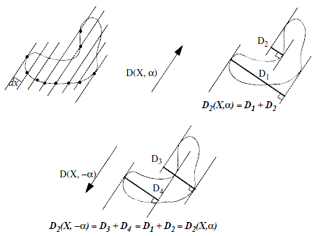
The Euler number is obtained as the sum of measures in local neighborhoods. In the continuous case, this measure is null almost everywhere, except on contours. An example illustrates this for polygonal shapes in the figure 1.
In the discrete case, the local measure, a search for specific configurations, is derived from the Euler formula for graph:  , where
  is the number of connected components,
  the number of holes,
  the number of vertices,
  the number of elementary faces, and
  the number of sides.
On a square grid, one gets:

For example, consider the Euler number in the following continuous case of a polygonal object with no loops, and bounding an object or a hole.
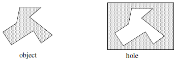 A simple local measure can identify this contour as the boundary of an object or a hole. We define a measure
  for each point
  in the plane as:
- if is a vertex then the value of
 is 0.
is 0.
- otherwise, consider the side normals.
Two situations may occur: the object points (shaded set) lie in the concavity or in the convexity.
 In the first case the measure will be defined as:
  , and in the second case as:
  , where
  is the angle, lying between 0 and
  , of the
  and
and  side normals, oriented toward the convexity.
The polygonal measure is then defined as: 
One can easily show that:
 if
if  is an object, and:
 if is a hole.
If several disjointed polygonal contours exist in an image, one can apply this measure on each contour, and obtain:  which gives the Euler formula.
In 3D, the Euler-Poincar
 is the number of objects (that is to say the number of connected components),
 the connectivity, and
 the number of enclosed cavities.
The Euler-Poincarformula for a 3D object  is given:
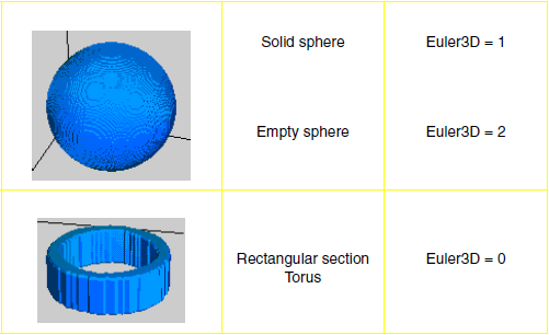 The Euler number is a characteristic of a three-dimensional structure which is topologically invariant (it remains unchanged by elastic transformations of the structure). It measures what might be called "redundant connectivity" - the degree to which parts of the object are multiply connected (Odgaard et al. 1993). It is a measure of how many connections in a structure can be severed before the structure falls into two separate pieces.
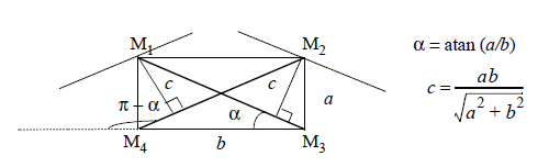
Feret's diameter is defined as the distance between two parallel tangents of a particle on a given direction like the measurement by a caliper (see Figure 4). This definition is extended to 3D with the distance between two tangent planes.
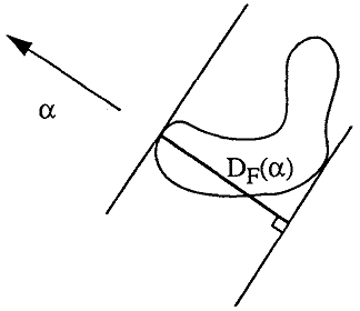
In 2D Feret's diameters are computed along all directions  which can determine the minimum, the mean and the maximum.
By default the distribution of Feret diameter is made up of a sampling of 10 angles from 0 to 162 degree with a step of 18 degree. This distribution can be customized with the Feret 2D angles attributes.
In 3D Feret diameter is a one-dimensional measurement that estimates how "wide" some segmented object is, when projected by a particular angle. The distance between the outermost tangents of the segmented object defines the diameter for that angle:
LENGTH_3Dis the longest Feret diameter.WIDTH_3Dis the shortest Feret diameter.FERET_DIAMETER_RATIO_3Dis the ratio between shortest Feret diameter and its normal Feret diameter.
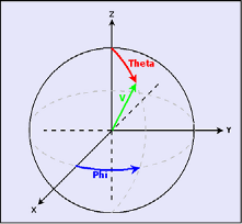
The 3D distribution is computed to get the predefined number of angles regularly spreaded around the upper part of the unit sphere. By default a sampling of 31 angles. This distribution can be customized with the Feret 3D angles attributes. The orientations are defined by the couple of angles from spherical coordinates 
 The direction given by the Feret diameters allows to defines four angles:
WIDTH_ORIENTATION_THETA_3Dis the Theta angle in spherical coordinate system of the shortest Feret diameter.WIDTH_ORIENTATION_PHI_3Dis the Phi angle in spherical coordinate system of the shortest Feret diameter.LENGTH_ORIENTATION_THETA_3Dis the Theta angle in spherical coordinate system of the shortest longest Feret diameter.LENGTH_ORIENTATION_PHI_3Dis the Phi angle in spherical coordinate system of the shortest longest Feret diameter.
The intercept count measurement is the number of entries in an object along a given direction.
Let's consider a set of lines  , parallel to a direction , and regularly spaced by
  .
.
The diametral variation is defined as:  Where
Where  is the number of boundary points which intersect the set of lines
  . This is equivalent to the sum of the lengths of the projections of the object in the direction.
Note that  is symmetric:
 The discrete case in 2D translates to the search for specific configurations, as defined in the table below.
The Crofton formula computes the perimeter using the intercept count.
Cauchy's formula shows that:  The perimeter is then approximated when the above integral is replaced by a discrete summation. In the square grid case, the summation is computed for the four fundamental directions:
  Where:
 represents the intercept count along the direction ,
-
a represents the distance between two points on the grid and the distance between two lines in the
 or
or  directions,
 is the distance between two lines in the
  and
and  directions.
Finally, this formula can be corrected for non square pixels. In such a situation, the diagonals no longer fit the and directions. Let  be the four neighbouring pixels on the grid,
a be the distance between horizontal lines,
b be the distance between vertical lines and
c the distance between diagonal lines.
be the four neighbouring pixels on the grid,
a be the distance between horizontal lines,
b be the distance between vertical lines and
c the distance between diagonal lines.
 The formula becomes:
A quantile value, associated to a given percentage of observations, is the value of the cumulative distribution at the given percentage.
Such a quantile value is computed by interpolation between the first bin where the cumulated histogram is higher than the percentage of observations and its previous bin.
The cumulated histogram is given at the center of each bin, counting the half population of the current bin. For instance with a bin size of 1, the cumulated histogram for the bin 3.. 4 is computed adding the total population of the values 0, 1 and 2 to the half population of the value 3. It is assigned to the bin center 3.5.
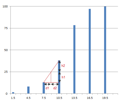 With the example above, where the bin size is 3, the 25% quantile value of the histogram is:
  Where :
-
Class Summary Class Description SoDataMeasure Abstract base class for all ImageViz image data measures.SoDataMeasureAttributes Class for all ImageViz data measure attributes.SoDataMeasureCustom class to define a custom measure.SoDataMeasurePredefined class that define the list of predefined measure that can be used on image data input. -
Enum Summary Enum Description SoDataMeasure.ResultFormats The "result format" is the type of the output of a measure computation.SoDataMeasure.UnitDimensions "Unit dimension" is used to categorize the resulting unit of a measure.SoDataMeasurePredefined.PredefinedMeasures Enumeration of all pre defined measure that can be used.