Introduction

More...

Classes
class	SoDataMeasure
	Abstract base class for all ImageViz image data measures. More...

class	SoDataMeasureAttributes
	Class for all ImageViz data measure attributes. More...

class	SoDataMeasureCustom
	class to define a custom measure. More...

class	SoDataMeasurePredefined
	class that define the list of predefined measure that can be used on image data input. More...

Detailed Description

Introduction

For instance, a set of measurements has to be selected using SoLabelAnalysisQuantification, SoLabelFilteringAnalysisQuantification or SoGlobalAnalysisQuantification engines. Here are described general priciples that help to understand most of the ImageViz predefined measurements.

The SoDataMeasurePredefined class contains the list of the measurements that are immediately available in ImageViz. Each measurement is identified by a PredefinedMeasure enumerate. The name of these enumerates may end with 2D or 3D:

2D indicates that a mesure is only supported with 2D images,
3D indicates that a measure is only supported with 3D images,
if this information is omitted, the measure works on both types of images.

Enumerates having a name starting with GRAY or INTENSITY are measurements based on the intensity image input.

These measures don't support intensity images with more than one channel. Please use the SoColorGetPlaneProcessing2d engine to extract the required channel before computing the intensity measurement.

Please see section Image Analysis to know how to perform analysis on such measurements.

Moment of inertia and covariance matrix

First order moments

In the continuous case they are defined as:

$M_{1x}=\frac{1}{A(X)}\int_X x \times g(x,y,z) \, dx \, dy \, dz$

$M_{1y}=\frac{1}{A(X)}\int_X y \times g(x,y,z) \, dx \, dy \, dz$

$M_{1z}=\frac{1}{A(X)}\int_X z \times g(x,y,z) \, dx \, dy \, dz$

and in the discrete case as:

$M_{1x} = \frac{1}{A(X)}\sum_{X}{x_i \times g(x_i,y_j,z_k)}$

$M_{1y} = \frac{1}{A(X)}\sum_{X}{y_j \times g(x_i,y_j,z_k)}$

$M_{1z} = \frac{1}{A(X)}\sum_{X}{z_k \times g(x_i,y_j,z_k)}$

Where $(x_i,y_j,z_k)$ is a point of the object X, g its gray level intensity and $A(X)$ the area of X.
For gray level images $A(X)=\sum_X{g(x_i,y_j,z_k)}$ , for binary images just consider $g(x_i,y_j,z_k)=1$ .
Note :

Name of ImageViz measurements based on these computations start with GRAY_ if the moments are computed weighting the result by the graylevels of the intensity image (e.g., GRAY_BARYCENTERX).
Other measurements don't take into account the graylevels of the intensity image (e.g., BARYCENTERX).
If the intensity image given to the analysis engine is a binary image, both types of measurement will output the same result (GRAY_BARYCENTERX = BARYCENTERX).

Second order moments

$M_{2x} = \frac{1}{A(X)}\sum_{X}{(x_i-M_{1x})^2 \times g(x_i,y_j,z_k)}$

$M_{2y} = \frac{1}{A(X)}\sum_{X}{(y_i-M_{1y})^2 \times g(x_i,y_j,z_k)}$

$M_{2z} = \frac{1}{A(X)}\sum_{X}{(z_i-M_{1z})^2 \times g(x_i,y_j,z_k)}$

$M_{2xy} = \frac{1}{A(X)}\sum_{X}{(x_i-M_{1x})(y_i-M_{1y}) \times g(x_i,y_j,z_k)}$

$M_{2xz} = \frac{1}{A(X)}\sum_{X}{(x_i-M_{1x})(z_i-M_{1z}) \times g(x_i,y_j,z_k)}$

$M_{2yz} = \frac{1}{A(X)}\sum_{X}{(y_i-M_{1y})(z_i-M_{1z}) \times g(x_i,y_j,z_k)}$

Variance-covariance matrix

$M= \left[ \begin{array}{ccc} M_{2x} & M_{2xy} & M_{2xz}\\ M_{2xy} & M_{2y} & M_{2yz}\\ M_{2xz} & M_{2yz} & M_{2z}\end{array}\right]$

The orientation is defined as the direction of its major inertia axis. It is given as the eigenvector of the largest eigenvalue of the covariance matrix.

This is a good measure of the orientation for simple, roughly convex objects.

The result $\theta$ falls between -180 and +180 degree.

The result $\varphi$ falls between 0 and 90 degree.

The secondary orientation (or orientation2) is defined as the direction of its minor inertia axis. It is given as the eigenvector of the smallest eigenvalue of the covariance matrix.

Extent values

Euler characteristic

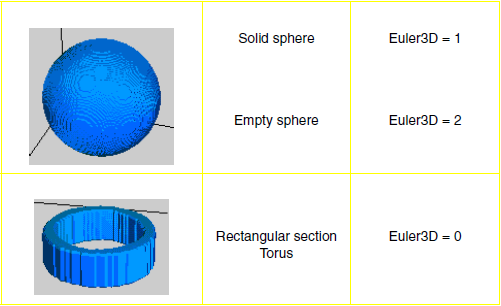
The Euler number, or connectivity factor $N_2(X)$ , is related to the number of connected components $N_C(X)$ , and to the number of holes $N_h(X)$ in each of these components. The Euler number is defined as $N_2(X)=N_C(X)-N_h(X)$ .

For objects with no hole, a very fast algorithm exists to compute the number of objects or components.

The Euler number is a topological parameter, which describes the structure of an object, regardless of its specific geometric shape. Other topological parameters exist, such as the number of branches or of triple points in a skeleton, the hierarchical degree of a tree-like skeleton or the number of neighbours for a cell in a skeleton by zone of influence.

The connectivity number $N_2(X)$ can be interpreted geometrically (Euler-Poincaré). The connectivity numbers $N_0(X)$ , $N_1(X)$ , are computed recursively when the spatial dimension increases. Details of this approach are beyond the scope of this documentation.

The Euler number is obtained as the sum of measures in local neighborhoods. In the continuous case, this measure is null almost everywhere, except on contours. An example illustrates this for polygonal shapes in the figure 1.

In the discrete case, the local measure, a search for specific configurations, is derived from the Euler formula for graph: $N_2(X)=c-h=v+f-s$ , where $c$ is the number of connected components, $h$ the number of holes, $v$ the number of vertices, $f$ the number of elementary faces, and $s$ the number of sides.

On a square grid, one gets:

$N_2(X)=N \left[\begin{array}{cc} 1 & 0\\ 0 & 0\end{array}\right]-N\left[\begin{array}{cc} . & 0\\ 1 & 0\end{array}\right]$

For example, consider the Euler number in the following continuous case of a polygonal object with no loops, and bounding an object or a hole.

Figure 1: Polygonal object

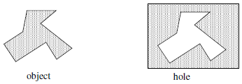
A simple local measure can identify this contour as the boundary of an object or a hole. We define a measure $m$ for each point $x$ in the plane as:

if is a vertex then the value of is 0.
otherwise, consider the side normals.

Two situations may occur: the object points (shaded set) lie in the concavity or in the convexity.

Figure 2: Concavity and convexity

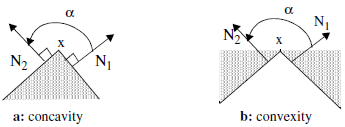
In the first case the measure $m$ will be defined as: $m(x) = \alpha$ , and in the second case as: $m(x) = -\alpha$ , where $\alpha$ is the angle, lying between 0 and $\pi$ , of the $N_1$ and $N_2$ side normals, oriented toward the convexity.

The polygonal measure is then defined as:

$m(P) = \sum_{s_i}m(s_i)~\mbox{, where $s_i$ are the polygonal vertices.}$

One can easily show that:

if is an object, and:
if is a hole.

If several disjointed polygonal contours exist in an image, one can apply this measure on each contour, and obtain:

$m(\cup P_i)=2\pi\times N_C - 2\pi\times N_t \mbox{,}$

which gives the Euler formula.

Euler characteristic for 3D objects

In 3D, the Euler-Poincaré number of the object is an indicator of the connectivity of a complex structure. The components of the Euler number are the three Betti numbers:

$\beta_0$ is the number of objects (that is to say the number of connected components),
$\beta_1$ the connectivity, and
$\beta_2$ the number of enclosed cavities.
The Euler-Poincaré formula for a 3D object is given:
$\chi(X)=\beta_0-\beta_1+\beta_2$

Figure 3: Euler number 3D examples
The Euler number is a characteristic of a three-dimensional structure which is topologically invariant (it remains unchanged by elastic transformations of the structure). It measures what might be called "redundant connectivity" - the degree to which parts of the object are multiply connected (Odgaard et al. 1993). It is a measure of how many connections in a structure can be severed before the structure falls into two separate pieces.

Feret's Diameter

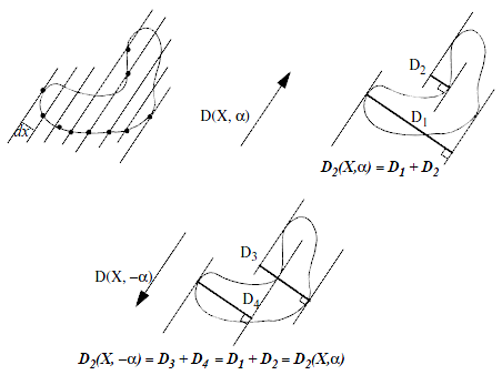
Feret's diameter is defined as the distance between two parallel tangents of a particle on a given direction like the measurement by a caliper (see Figure 4). This definition is extended to 3D with the distance between two tangent planes.

Figure 4: Feret's diameter

2D Feret's diameter

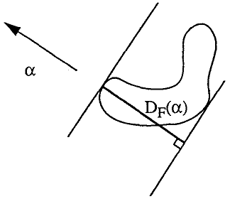
By default the distribution of Feret diameter is made up of a sampling of 10 angles from 0 to 162 degree with a step of 18 degree. This distribution can be customized with the Feret 2D angles attributes.

2D Feret's diameter

In 3D Feret diameter is a one-dimensional measurement that estimates how "wide" some segmented object is, when projected by a particular angle. The distance between the outermost tangents of the segmented object defines the diameter for that angle:

LENGTH_3D is the longest Feret diameter.
WIDTH_3D is the shortest Feret diameter.
FERET_DIAMETER_RATIO_3D is the ratio between shortest Feret diameter and its normal Feret diameter.

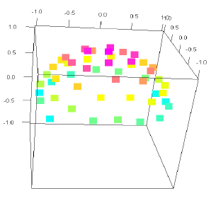
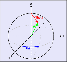
The 3D distribution is computed to get the predefined number of angles regularly spreaded around the upper part of the unit sphere. By default a sampling of 31 angles. This distribution can be customized with the Feret 3D angles attributes. The orientations are defined by the couple of angles from spherical coordinates $( \theta, \phi )$

Figure 5: Example of a distribution of 3D angles

The direction given by the Feret diameters allows to defines four angles:

WIDTH_ORIENTATION_THETA_3D is the Theta angle in spherical coordinate system of the shortest Feret diameter.
WIDTH_ORIENTATION_PHI_3D is the Phi angle in spherical coordinate system of the shortest Feret diameter.
LENGTH_ORIENTATION_THETA_3D is the Theta angle in spherical coordinate system of the shortest longest Feret diameter.
LENGTH_ORIENTATION_PHI_3D is the Phi angle in spherical coordinate system of the shortest longest Feret diameter.

Figure 6: Azimuthal and polar angles

Intercept count

Diametral variation

$D_2(X,\alpha)=\int{N_\alpha(X)dx}$

Where $N_\alpha(X)$ is the number of boundary points which intersect the set of lines $d(x,\alpha)$ . This is equivalent to the sum of the lengths of the projections of the object in the $\alpha$ direction.

Note that $D_2(X,\alpha)$ is symmetric:

Figure 7: Application of the diametral variation formula

The discrete case in 2D translates to the search for specific configurations, as defined in the table below.

$\begin{array}{|c|c|} \hline 0 & \begin{array}{ccccc} \mbox{x} & & \mbox{x} & & \mbox{x}\\ \mbox{x} & & 0 & & 1\\ \mbox{x} & & \mbox{x} & & \mbox{x} \end{array}\\ \hline 45 & \begin{array}{ccccc} \mbox{x} & & \mbox{x} & & 1\\ \mbox{x} & & 0 & & \mbox{x}\\ \mbox{x} & & \mbox{x} & & \mbox{x} \end{array}\\ \hline 90 & \begin{array}{ccccc} \mbox{x} & & 1 & & \mbox{x}\\ \mbox{x} & & 0 & & \mbox{x}\\ \mbox{x} & & \mbox{x} & & \mbox{x} \end{array}\\ \hline 135 & \begin{array}{ccccc} 1 & & \mbox{x} & & \mbox{x}\\ \mbox{x} & & 0 & & \mbox{x}\\ \mbox{x} & & \mbox{x} & & \mbox{x} \end{array}\\ \hline \end{array}$

Crofton perimeter

$L(X)=\int_{0}^{\pi}D_2(X,\alpha)d\alpha$

The perimeter is then approximated when the above integral is replaced by a discrete summation. In the square grid case, the summation is computed for the four fundamental directions:

$L(X)=\frac{\pi}{4}\times [a \times(N_0+N_{90})+\frac{a}{\sqrt2}\times(N_{45}+N_{135}) \right ]$

Where:

$N_\alpha$ represents the intercept count along the direction $\alpha$ ,
a represents the distance between two points on the grid and the distance between two lines in the $0^\circ$ or $90^\circ$ directions,
$\frac{a}{\sqrt2}$ is the distance between two lines in the $45^\circ$ and $135^\circ$ directions.

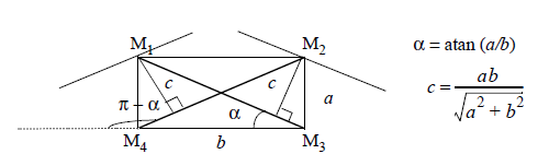
Finally, this formula can be corrected for non square pixels. In such a situation, the diagonals no longer fit the $45^\circ$ and $135^\circ$ directions. Let $M_i$ be the four neighbouring pixels on the grid, a be the distance between horizontal lines, b be the distance between vertical lines and c the distance between diagonal lines.

Figure 8: Crofton perimeter on non-square pixels

The formula becomes:

$L(X)=\alpha \times a \times N_0 + (\frac{\pi}{2}-\alpha)\times b \times N_{90} + \frac{\pi}{4}\times c \times (N_{\alpha}+N_{\pi-\alpha})$

Quantile of an histogram

Such a quantile value is computed by interpolation between the first bin where the cumulated histogram is higher than the percentage of observations and its previous bin.

The cumulated histogram is given at the center of each bin, counting the half population of the current bin. For instance with a bin size of 1, the cumulated histogram for the bin 3.. 4 is computed adding the total population of the values 0, 1 and 2 to the half population of the value 3. It is assigned to the bin center 3.5.

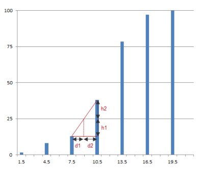
Figure 9: Histogram quantile interpolation

With the example above, where the bin size is 3, the 25% quantile value of the histogram is:

$Q(25) = \lambda \times 7.5 + (1- \lambda) \times 10.5$

Where :

$\lambda = \frac{d2}{(d1+d2)} = \frac{h2}{(h1+h2)}$

Open Inventor Release 2023.2.3

Introduction

Classes

Detailed Description

Introduction

Moment of inertia and covariance matrix

First order moments

Second order moments

Variance-covariance matrix

Extent values

Euler characteristic

Euler characteristic for 3D objects

Feret's Diameter

2D Feret's diameter

2D Feret's diameter

Intercept count

Diametral variation

Crofton perimeter

Quantile of an histogram