Your job as programmer is to define the components that make up the parametric functions, referred to as f(), g(), and h() in the previous section. Instead of explicitly specifying the equations, you specify the following three things:
Control points are points in object space that affect the shape of the curve in some way. The curve may pass near the control points, as shown at the left in Using Control Points to Shape the Curve , or pass through some of them, as shown at the right in the figure. The control points can be a set of data points through which you want to fit a curve, or a grid of points used to describe a curved surface such as the hood of a car. In Inventor, control points are specified in an SoCoordinate3 or SoCoordinate4 node.

The knot sequence defines how the control points affect the curve. The knot sequence is simply a list of nondecreasing numbers. These numbers determine whether the curve passes through and interpolates between some of the control points (an interpolating curve) or passes near the control points (an approximating curve). In Inventor, the knot sequence is specified in an SoNurbsCurve or SoNurbsSurface (or SoIndexedNurbsCurve, SoIndexedNurbsSurface) node.
The order of a curve determines the form of the parametric equations. The order is equal to one plus the maximum exponent (degree) of the variables in the parametric equations. For example, the parametric equations of a cubic curve (degree = 3, order = 4) have the following form:
Similarly, the parametric equations of a quadratic curve (degree = 2, order = 3) have the following form:
Alternatively, you may wish to think of the order as the number of coefficients in the parametric equation. The order of a curve affects how smooth the curve can be (see Continuity of a Curve).
In Inventor, the order of a curve is not explicily specified. Order is equal to
number_of_knots - number_of_control_points
The order of the curve determines the minimum number of control points necessary to define the curve. You must have at least order control points to define a curve. (So for a curve of order 4, you must have at least four control points.) To make curves with more than order control points, you can join two or more curve segments into a piecewise curve (see Piecewise Cubic Curve ).
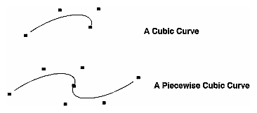
The order of the curve also affects how the curve behaves when a control point is moved. In Inventor, a NURBS curve can have an order up to 8. However, higher orders introduce oscillation into the curve and can behave unpredictably when a control point moves. Cubic curves (order of 4) are the most commonly used curves, since they provide enough control for most geometric modeling applications without the drawbacks of higher-order curves.
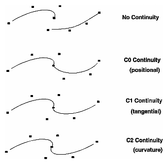
A breakpoint is where two curve segments meet within a piecewise curve. The continuity of a curve at a breakpoint describes how those curves meet at the breakpoint. Continuity of a Curve shows four possible types of continuity:
| No continuity | The curves do not meet at all. |
| C 0 continuity | The endpoints of the two curves meet (the curves have positional continuity only). There may be a sharp point where they meet. |
| C 1 continuity | The curves have identical tangents at the breakpoint. (The tangent is the slope at the breakpoint.) The curves join smoothly. C1 curves also have positional continuity. |
| C2 continuity | The curves have identical curvature at the breakpoint. (Curvature is defined as the rate of change of the tangents.) Curvature continuity implies both tangential and positional continuity. |
The order of a curve determines the maximum continuity possible. Thus, you may need a higher order curve if you need more continuity. The maximum continuity is order - 2. For example, for cubic curves, the maximum continuity possible is C2 (curvature continuity).
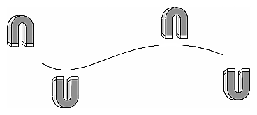
Each control point is like a magnet tugging on the curve (see Control Points Influence the Curve ). The strength and extent of these magnets is described mathematically by a particular basis function. For a NURBS, this function is the B-spline basis function. (See Suggestions for Further Reading for references presenting a more thorough derivation of the B-spline basis function.)
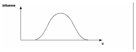
The B-spline basis function (B-Spline Basis Function ) describes the curve in parameter (u) space. For each value of u:
contribution_of_each_control_point = location * its_basis _function
The resulting curve is equal to the sum of the contributions from each control point. Note that often a control point (a “magnet”) affects the entire curve, although its influence becomes weaker as you move away from it. The exact extent of the influence is determined by the knot sequence.
The distribution of basis functions in parameter space is controlled by the knot sequence (also referred to as the knot vector, or the knots). The knot sequence is a list of nondecreasing values. Each knot defines the beginning and end of a basis function. There must be exactly *(order + number of control points)* values in the knot sequence. The curve is defined only where order basis functions overlap (as shown in Uniform Knot Sequence ). If the knot values are singular (no repeating values) and regularly spaced, the curve is a uniform B-spline (as shown in Uniform Knot Sequence ).
Uniform Knot Sequence shows a uniform knot sequence. Four control points are defined (in object space). The top of the figure illustrates the four basis functions for each of the control points. The basis functions overlap where u = 3.0 to u = 4.0, as indicated by the shaded portion. This figure also illustrates another important NURBS relationship: at any point where the curve is defined, the sum of all basis functions is equal to 1.
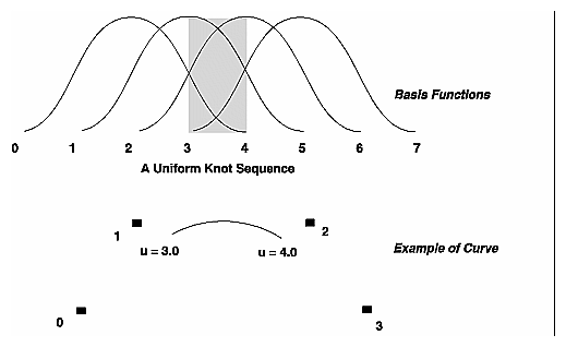
Distinct knot values define segments. A basis function always spans order segments. In Uniform Knot Sequence , for example, the basis function beginning at 0 and ending at 4 spans four segments (knot 0 to knot 1; knot 1 to knot 2; knot 2 to knot 3; and knot 3 to knot 4).
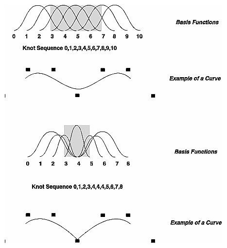
Duplicating values in the knot sequence increases that value's multiplicity and causes more than one basis function to start at that point. This also causes a corresponding decrease in the continuity of the curve. Knot Multiplicity uses the same two sets of control points, with different knot sequences for the top and bottom curves. Notice how the bottom curve has C0 continuity, and the top curve has C2 continuity. This relationship between multiplicity and the continuity of the curve can be expressed mathematically as follows:
where ORD equals the order of the curve and M is the multiplicity.
The maximum multiplicity (maximum times you can repeat a knot) is order. Continuity_and_Knot_Multiplicity_for_Cubic_Curves “Continuity and Knot Multiplicity for Cubic Curves” shows knot multiplicity and the resulting continuity.
Continuity and Knot Multiplicity for Cubic Curves
| Knot Multiplicity | Continuity Conditions | Continuity |
|---|---|---|
| 1 | positional tangential curvature | C2 |
| 2 | positional tangential | C1 |
| 3 | positional | C0 |
| 4 | none | none |
Several common knot sequences are extremely useful for a wide variety of applications:
| Uniform cubic B-spline | knots are uniformly spaced; single multiplicity (for example, 0, 1, 2, 3, 4, 5, 6, 7) |
| Cubic Bezier curve | multiplicity = 4 at beginning and end(for example, 0, 0, 0, 0, 1, 1, 1, 1) |
| Uniform cubic B-spline that passes through endpoints | multiplicity= 4 at beginning and end; uniformly spaced single knots between (for example, 0, 0, 0, 0, 1, 2, 3, 4, 5, 5, 5, 5) |
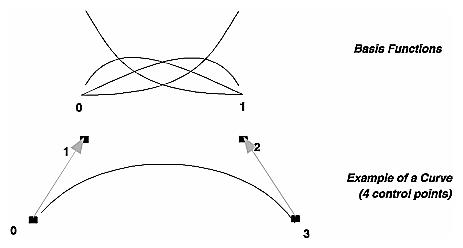
The behavior of the Bezier curve and the uniform cubic B-spline makes them ideal for geometric modeling and CAD applications. The curve passes through the first and last control points (see Cubic Bezier Curve ). A line drawn through the first and second control points determines the tangent at the first endpoint. A line drawn through the last two control points determines the tangent at the second endpoint.
The previous pages have outlined important relationships among NURBS parameters. They can be summarized as follows:
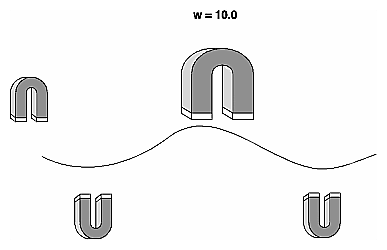
Each control point has an associated weight that influences the shape of its basis function. As shown in Rational Curves , this is analogous to having magnets of differing sizes tugging on the curve. For nonrational curves, all control points have a weight of 1.0. For rational curves, the control points have differing weights. If a control point has a weight greater than 1.0, its influence on the curve is greater than that of control points with weights of 1.0.
The parametric equations for rational curves have both a numerator and a denominator, which results in a ratio. (The numerator is the original parametric equation. The denominator is another parametric equation that takes the weight into account.) We recommend that the weight be a value greater than 0. Use an SoCoordinate4 node to specify x, y, z, and w (weight) values.
Rational curves and surfaces are required to accurately represent conic sections, spheres, and cylinders. For more information, see Suggestions for Further Reading.
If you've made it this far into the discussion of the NURBS, you now understand all the buzzwords that form this acronym:
| Non-Uniform | Knot spacing need not be uniform. |
| Rational | The parametric equations describing the curve can have a denominator (that is, they can be ratios). |
| B-Spline | The influence of the control points is based on the B-spline basis function. |