The MiCell( C++ | Java ) interface allows you to define 1D/2D/3D non linear cells. A cell is non linear when interpolation along the cell’s edges are not linear. The following conditions are necessary to define non linear cells for MeshViz:
Define additional nodes in the cell.
Define shape functions for each node of this cell.
Note for specialists in finite element methods:
MeshViz supports any iso-parametric element: MeshViz uses the same shape function to interpolate the geometry of the cell and to interpolate any other dataset.
MeshViz does not support non-iso-parametric elements because only one shape function is defined per cell’s node.
MeshViz supports Lagrange finite element type.
MeshViz does not support Hermite finite element type.
MeshViz supports serendipity finite element type. (no additional node inside the cell)
MeshViz supports any order of element (linear, quadratic, cubic, quartic …). MeshViz provides implementation of linear and quadratic shape functions of the most usual 1D, 2D and 3D finite elements. (triangle, quadrangle, tetrahedron, hexahedron, prism, pyramid). However the genericity of MeshViz allows you to implement easily other order of shape function (cubic …)
MeshViz supports un-complete finite element: usually the number of additional nodes is the same on each cell’s edge. Un-complete finite elements are elements where the number of additional nodes is not constant per edge: for instance a triangle of 4 nodes with just one additional node on one edge.
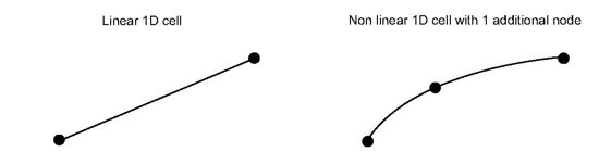
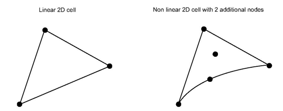
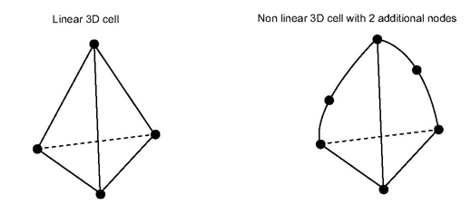
For 1D cells, additional nodes are along the edge. For 2D cells, additional nodes are on the edges and/or inside the cell. For 3D cells, additional nodes are on the edge, and/or inside the face of the cell and/or inside the cell.
Example of additional nodes
The number of additional nodes per edge defines the order of the cell:
A cell is linear when each edge has 2 nodes.
A cell is quadratic when each edge has 3 nodes.
A cell is cubic when each edge has 4 nodes.
A cell is quartic when each edge has 5 nodes.
Etc…

Additional nodes are also usually defined inside the cell for cubic element (see figure above) but also so for quadratic rectangular base shape:
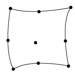
However, MeshViz can also handle elements without these interior additional nodes (serendipity element).
![[Tip]](../../images/tip.jpg) | |
Note: Shape functions are also often called interpolation functions or weight functions. MeshViz define them in the MiCell interface by the method getWeight(). |
Shape functions define the way to interpolate in the cell, thus defining the shape of the cell. They are expressed as parametric functions with 1, 2 or 3 parameters. These parameters are called the parametric coordinates of a point in the cell. The parametric coordinates are always expressed in a constant interval (usually [0-1]) called the normalized space.
Property 1:
A shape function must be defined for each node of the cell. For instance the non linear triangle of 5 nodes as shown in the previous figure must define exactly 5 shape functions of 2 parameter (r,s)
Property 2:
The value of the shape function fi must be 1 for the i-th node of the cell and 0 for any other node. Thus
fi (rj, sj, tj) = 1 for j = i = 0 for j ≠ i
where (rj, sj, tj) are the parametric coordinates of the j-th node of the cell.
Property 3:
The sum of the shape functions must always be 1 whatever the value of the parametric coordinates. Thus
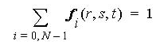
where N is the number of nodes of the cell, and whatever the parametric coordinates (r,s,t)
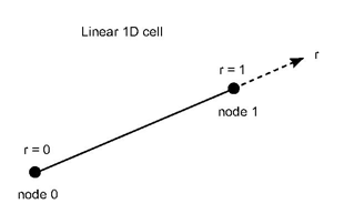
The shape functions for a 1D linear cell (a simple edge of 2 nodes) can be
f0 (r) = 1-r
f1 (r) = r
where r belongs to the interval [0-1] for each point between the 2 nodes.
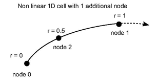
The shape functions for a 1D quadratic cell (here a “curve” edge of 3 nodes) can be
f0 (r) = 2(r-0.5)(r-1)
f1 (r) = 2r(r-0.5)
f2 (r) = 4r(1-r)
where r belongs to the interval [0-0.5] for each point between the nodes 0 and 1 and belongs to the interval [0.5-1] for each point between the nodes 1 and 2.
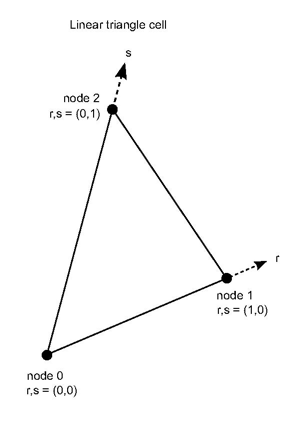
The shape functions for a 2D linear triangle cell can be:
f0 (r,s) = 1-r-s
f1 (r,s) = r
f2 (r,s) = s
where (r,s) = (0,0) at node 0, (1,0) at node 1 and (0,1) at node 2.
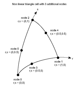
The shape functions for a 2D quadratic triangle cell with 1 additional node on each edges can be:
f0 (r,s) = (1-r-s) * ( 2*(1-r-s)-1 )
f1 (r,s) = r * (2*r-1)
f2 (r,s) = s * (2*s-1)
f3 (r,s) = 4 * r * (1-r-s)
f4 (r,s) = 4 * r * s
f5 (r,s) = 4 * s * (1-r-s)
where (r,s) = (0,0) at node 0, (1,0) at node 1 and (0,1) at node 2,(0.5,0) at node 3, (0.5,0.5) at node 4 and (0,0.5) at node 5.
| |
Note: MeshViz and the MiCell interface do not assume anything about the ordering of the additional nodes in a non linear cell. In the previous images the additional node numbers follow the linear node number but it is just an example of numbering. It is up to the application to choose the cell’s node numbering but the value of the shape functions must be defined according to this numbering. |
To interpolate data to a point P inside a cell (linear or not) from the node of the cell, we need:
The parametric coordinates of the point P.
The value of the shape functions at P.
The data value at each node of the cell
The interpolated data is a linear combination of the shape functions at P and the data value at each node of the cell:
Formula 1
For 1D cell

For 2D cell

For 3D cell

where dr,s,t is the interpolated data of the point having parametric coordinates (r,s,t) and di is the data of the i-th node of the cell.
The previous formulas are the general form for data interpolation in cells when the data is defined at cell nodes and whatever the data type. Thus we use the same formula for scalar, vector, tensor values.
When the data is defined per cell, no interpolation is done thus:
Formula 2
dr, = dc
dr = dc
dr,s,t = dc
whatever the value (r,s,t) and where dc is the data at the cell containing the point (r,s,t)
Probing means finding the value of any point in the space using the discrete values given per node or per cell. Probing needs two steps:
Find the cell of the mesh that contains the position of the probe
Compute the value at the probe by using the found cell and either formula 1 or formula 2.
Like for interpolation, if the dataset being probed is per node, the second step needs to compute the shape functions of the probe position in the found cell. Furthermore the first step often needs to also compute the shape functions.
By definition coordinates data are always defined per node, so formula 1 is always used to interpolate coordinates in a non linear cell. Thus the shape functions are also used to draw the cell because graphic libraries (and the graphics board) always assume that edges and faces are linear. Actually, drawing using shape functions is equivalent to going from the normalized space to the world coordinate space:
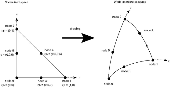
Each point (r,s) in the normalized space is transformed by formula 1 to get its world coordinates.
As graphic board and graphic libraries are not able to directly handle non linear edges and surfaces, if we just transform the nodes of the non linear cell by formula 1, we would obtain a result somethng like the following one:
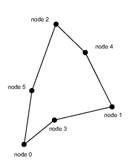
It could be "good enough" if this non linear triangle is very small compared to the screen area. But it is far from the real shape of that triangle as shown in the previous section. In order to enhance the rendering, we introduce new points in the normalized space inside, on the face or on the edges of the non linear cell. We can easily compute the parametric coordinates of these new points by doing a linear interpolation of the parametric coordinates of the cell’s node. Then we use formula 1 to get the real coordinates of these new points in the world coordinate space.
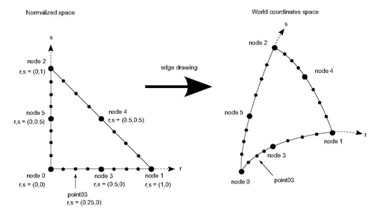
Figure 8 shows how the introduction of new points on the cell edge of the normalized space enhances the rendering of this non linear triangle cell. Of course the segments used to join the new points are still straight segments and the result is still an approximation of the non linear triangle. The quality of the approximation depends on the number of new points introduced.
We call tessellation the step of introducing new points to build smaller sub-regions of non linear cells. When drawing the edges of a 1D, 2D or 3D cell, we just need to introduce new points on the edges starting from the normalized cell (see fig 8). When drawing a 2D cell or one face of a 3D cell we also need to introduce new points and new triangles inside the selected face (see point p34, p35, p45 in the following figure).
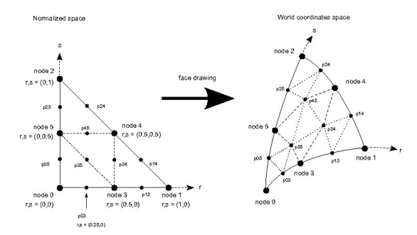
Thus the tessellation must be able to do at least two main tasks:
Tessellate lines by introducing new points on the edges of the cell
Tessellate faces by introducing sub triangles and new points on the edges and inside the cell.
The sub regions must be as small as possible so that we can assume they have almost linear properties. However we must keep in mind that passing from the normalized space to the world coordinate space is time consuming because it requires calling all the shape functions for each node of the cell. For instance, if the tessellation of a triangle cell of 6 nodes introduces 10 new points, at least 60 calls to the shape functions are done.
| |
Note: Tessellation is only used when drawing: it is not needed to probe or to interpolate. |
The tessellation step is exposed in the MeshViz API via the MiTessellator( C++ ) interface.
MeshViz extractor classes for unstructured meshes use an optional instance of MiTessellator( C++ ) to correctly handle the non linear cells. For instance to extract the skin of an unstructured mesh we must build a new instance of the extractor like this:
C++
skinExtract = MiSkinExtractUnstructured::getNewInstance (mesh, true, tessellator);
The last argument is optional and must be either the null pointer or an instance of the MiTessellator( C++ ) interface. When giving the null pointer, the mesh is assumed to be linear and no tessellation is done. Thus if the mesh contains for instance some triangle cells with 6 nodes, MeshViz will generate an output like in Figure 2.27, “ Untesselated quadratic shape”.
This MiTessellator( C++ ) interface has the following main methods:
start/finishVolumeTessellation
tessellateVolumeCell
start/finishSurfaceTessellation
tessellateSurfaceCell
start/finishLineTessellation
tessellateLineCell
When giving an instance of the MiTessellator( C++ ) interface, this tessellator is used for each extracted line or surface of the input mesh. For instance when calling
skinExtract->extractSkin(…);
the method tessellator->tessellateSurfaceCell(…) is called for each face of the skin mesh.
Thus the pseudo code to extract a surface from a non linear unstructured mesh is:
C++
extractSurface(...)
{
Extract the surface
  startSurfaceTessellation()
  For each surfaceCell extracted
  {
  tessellateSurfaceCell(surfaceCell)
  }
finishSurfaceTessellation()
}
In the same way, the pseudo code to extract a line from a non linear unstructured mesh is:
C++
extractLine(...)
  {
  Extract the line
    startLineTessellation()
    For each lineCell extracted
    {
    tessellateLineCell(lineCell)
    }
  finishLineTessellation()
  }
MiTessellator( C++ ) is an interface with only pure virtual methods. The MeshViz extractor does not know the actual instance of this interface that was chosen.. This mechanism allows advanced applications to write their own tessellator, provided this custom tessellator implements correctly all the methods of MiTessellator( C++ ).
Of course MeshViz provides a built-in tessellator that can be retrieved using a factory method of MiTessellator( C++ ):
C++
getNewTessellatorGeometry (const MiEdgeErrorMetric< MbVec3d > &edgeMetric)
This method returns a new instance of an internal implementation of MiTessellator( C++ ) which takes into account the geometry of the mesh and the given edgeMetric criterion. Note that this built-in geometry tessellator does not take into account any data set to make the tessellation. Thus the resulting tessellation is independent of any mapped dataset, and some color artifacts may appear.
The edge metric criterion is another interface with just one method
C++
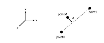
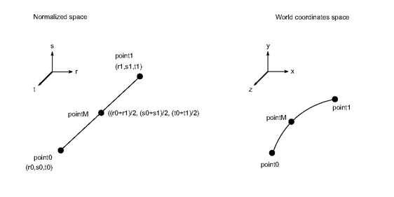
bool isEdgeLinear(point0, point1, pointM)
This method must check if an edge can be considered as linear or not according to the 3 coordinates point0, point1, pointM. Point0 and point1 are the endpoints of the edge and pointM is the real coordinate corresponding to the associated middle point in the normalized space (See the following figure).
An advanced application can easily create a custom implementation of MiEdgeErrorMetric( C++ ) by computing a custom geometry criterion. Note that the method isEdgeLinear() must be symmetric, thus:
C++
isEdgeLinear(point0, point1, pointM)
must return the same result as
C++
isEdgeLinear(point1, point0, pointM)
MeshViz provides a built-in implementation of the MiEdgeErrorMetric( C++ ) interface: the class MxEdgeErrorMetricGeometry implements the interface MiEdgeErrorMetric( C++ ) by using a maxError distance. MxEdgeErrorMetricGeometry::isEdgeLinear(…) returns true if the distance d from pointM to the edge [point0, point1] is less than maxError. (See the following figure)