 The GraphMaster class library extends Open Inventor capabilities in the following three areas:
- 2D drawing : With this first set of extensions, you can design your 2D graphics applications very easily and efficiently. This includes simple 2D shapes, such as rectangles, circles, and arrows, 2D charting nodes to draw a large range of different 2D axes (linear, logarithmic, angular, time, etc.), curves and markers fields, statistical nodes using pie or bar chart representations, error areas, high-low-close curves, and so forth.
- 3D drawing : The previous classes are extended to 3D in order to provide features such as 3D circles, 3D pie or bar charts, 3D curves, and 3D axes. These nodes give you access to a wide range of new 3D functionality.
- Legends : A wide variety of legends is provided to annotate your visualizations. Before going any further, it is very important to read What You Must Know about MeshViz XLM:, mainly for the reminder about node kits and the explanation of the GraphMaster and 3DdataMaster domain facilities.
Simple 2D and 3D Nodes
GraphMaster introduces the following 2D and 3D classes that complement the Open Inventor 3D shape node set:
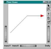
Example : Drawing an arrow
// tutorialGraph01.cxx
...
// Create the root of the scene graph
SoAnnotation* root = new SoAnnotation;
root->ref();
// Create the arrow and set appearance
PoArrow* myArrow = new PoArrow;
SbVec2f points[3] = { SbVec2f( 0., 0. ), SbVec2f( 10., 10. ), SbVec2f( 20., 10. ) };
myArrow->point.setValues( 0, 3, points );
myArrow->endPatternType = PoArrow::DIRECT_TRIANGLE;
myArrow->set( "endApp.material", "diffuseColor 1 0 0" );
myArrow->set( "appearance.material", "diffuseColor 0 0 0" );
myArrow->patternWidth = .1;
myArrow->patternHeight = .075;
// Set the domain to define end pattern size
#ifdef USE_PB
PbDomain myDom( 0., 0., 20., 20. );
myArrow->setDomain( &myDom );
#else
PoDomain* myDom = new PoDomain;
myDom->min = SbVec3f( 0, 0, 0 );
myDom->max = SbVec3f( 20, 20, 0 );
root->addChild( myDom );
#endif
root->addChild( myArrow );
SoXtPlaneViewer* viewer = new SoXtPlaneViewer( myWindow );
viewer->setSceneGraph( root );
viewer->setBackgroundColor( SbColor( 1., 1., 1. ) );
...
Business Graphics Nodes
Class tree
GraphMaster provides the following 2D and 3D classes that give you access to a whole new set of features for designing business graphics visualizations, such as curves, high-low-close curves, error bars, axes and axis systems, bar charts, legends, and more. (The indentation shows class derivations; you will notice that all classes are derived from PoGraphMaster ):
"Important"
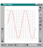
PoCurve and PoCurve3 are the two classes used to draw curves in 2D or 3D. PoCurve builds a curve in the XY plane and may use different representations depending on the curveRep field. This representation may be a standard polyline joining the given points, a smooth curve, a stair curve, etc. The area between the curve and a given threshold may be filled. “Raised” points can be added to the visualization, as well as markers to identify the location of points on the curve. The 3D class PoCurve3 only supports polyline and smooth representations.
The following example (located in $OIVHOME/src/MeshViz/Mentor) creates a curve (sine curve) and shows different attributes that can be used to change the visualization:
Example : A curve and its attributes 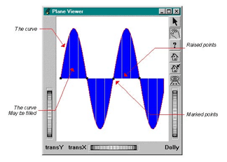
// tutorialGraph02.cxx
...
// Create the root of the scene graph
SoAnnotation* root = new SoAnnotation;
root->ref();
// Create the curve
PoCurve* myCurve = new PoCurve;
#define N_PT 50
#define PI 3.1415
SbVec2f points[N_PT];
double ang;
int i;
for ( i = 0, ang = 0.; i < N_PT; i++, ang += 4. * PI / ( double )N_PT )
points[i].setValue( ang, 6. * sin( ang ) );
myCurve->point.setValues( 0, N_PT, points );
myCurve->curveRep = PoCurve::CURVE_POLYLINE;
myCurve->isCurveFilled = TRUE;
myCurve->raiseFilterType = PoCurve::X_PERIOD;
myCurve->raiseXPeriod = PI / 3.;
myCurve->raiseThreshold = 0.0;
myCurve->markerFilterType = PoCurve::X_PERIOD;
myCurve->markerXPeriod = PI;
myCurve->set( "markerApp.material", "diffuseColor [0 0 0]" );
myCurve->set( "markerApp.drawStyle", "pointSize 5.0" );
myCurve->set( "curvePointApp.material", "diffuseColor [1 0 0]" );
myCurve->set( "curveFillingApp.material", "diffuseColor [0 0 1]" );
root->addChild( myCurve );
SoXtPlaneViewer* viewer = new SoXtPlaneViewer( myWindow );
viewer->setSceneGraph( root );
viewer->setBackgroundColor( SbColor( 1., 1., 1. ) );
...
Step 2: A curve with its axis system
Axis Type
Now, we may want to add axes to our curve in order to make the visualization more meaningful. GraphMaster provides a wide range of axes: Cartesian, polar or angular, linear, logarithmic, generalized, and time axes. GraphMaster also provides axis system nodes that are able to maintain “boxes” of 2, 3, 4, or 6 axes, or sets of axes where axes are defined on a parallelepiped related to the view. The axis classes are as follows (indentation shows class derivations):
Axis node classes


* PoPolarLinAxis
* PoPolarLogAxis
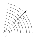
All axes will be drawn using a default representation if none is specified by the application. This means that depending on the domain, GraphMaster will compute the tick locations, text height, and so on, in order to generate a good default visualization.
 If necessary, you can change all the attributes of these axes, such as to suppress the arrow at the end, show a grid, add sub-graduations, change the label location, etc. You can do all this in your application by applying the different methods of PoAxis or derived classes.
Main axis attributes
The following picture shows the main axis attributes and axis terminology:
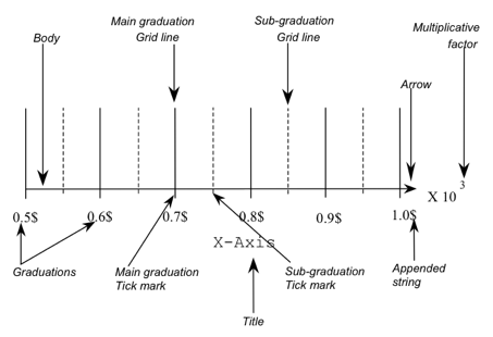
Main axis attributes
Graduation attributes
- gradVisibility : to switch graduation visibility on and off.
- gradPosition : to draw graduations above or below the axis.
- gradPath : to set the graduation path to be up, down, left, or right.
- gradFontName : to change the default font used to draw graduations.
- gradFontSize : to change the text height.
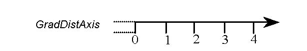 gradDistAxis : to specify the spacing between the graduations and the axis main line (relative to the domain).
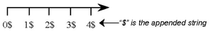 gradAddStringVisibility : an appended string may be added to each graduation (to specify a unit, for example).
- gradAddString : definition of the appended string.
Margin attributes
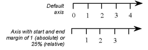 marginType : to specify if the following two margins are relative (% of axis length) or absolute (according to axis start and end fields).
- marginStart : margin between start point of the axis and first graduation.
- marginEnd : margin between end point of the axis and last graduation.
Title attributes
- titleVisibility : to switch the title visibility on and off.
- titlePosition : to draw the title in the middle or at the end of the axis.
- titlePath : to set the title path to be up, down, left, or right.
- titleFontName : to change the default font used to draw the title.
- titleFontSize : to change the text height.
- titleDistAxis : to specify the spacing between the title and the axis main line (relative to the domain).
- titleString : to specify the title string.
Grid line attributes
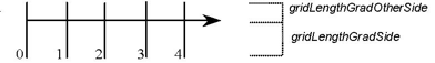 gridVisibility : to switch grid visibility on and off.
- gridLengthGradSide : to set the grid length on the graduation side. This length is specified relative to the domain.
- gridLengthGradOtherSide : to set the grid length on the side opposite the graduations. This length is specified relative to the domain.
Arrow attributes
- arrowVisibility : to switch arrow visibility on and off
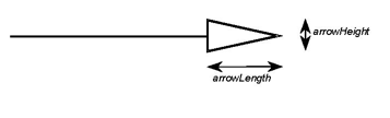 arrowHeight : to specify the arrow height relative to the domain.
- arrowLength : to specify the arrow length relative to the domain.
Tick mark attributes
- tickVisibility : to turn tick visibility on and off.
- tickPosition : to specify which side of the axis ticks are to be drawn on.
- tickMainLength : tick line length (relative to the domain).
- tickSubLength : sub-tick line length (relative to the domain).
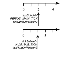 tickSubDef : to specify if tickNumOrPeriod field indicates the number of sub-graduations between two main graduations (NUM_SUB_TICK) or the period used to draw the graduations associated with the main tick (PERIOD_MAIN_TICK).
- tickNumOrPeriod : to define the value associated with the previous field. If tickSubDef is NUM_SUB_TICK and tickNumOrPeriod is 2, then two sub-ticks are drawn between two subsequent main ticks. If tickSubDef is PERIOD_MAIN_TICK and tickNumOrPeriod is 3, then no sub-ticks are drawn and only one main tick every three main ticks will be annotated with a graduation.
- tickFirstGrad : index of the first graduation to be drawn.
- tickLastGrad : index of the last graduation to be drawn.
Other attributes
- reverseFlag: using all current attributes, if this flag is on, then all character strings will be reversed (i.e., mirrored) before they are drawn.
GraphMaster objects are node kits (see the section called “Visualization classes”), so you can access each part and change the appearance of each of them. Many
axis attributes are computed relative to the domain (see What You Must Know about MeshViz XLM:). Text height, arrow length and width, number of ticks, height of ticks, etc. are
all computed automatically by GraphMaster (if the field is <= 0.) relative to the domain
if your application does not provide a value. All Cartesian and polar axes have geometric
starting and ending points. These points are used to compute the location of the axes on
the display. For an angular axis, the axis is always centered, when built, at point
(0,0,0).
Curve and axis merge examples
The following example (located in $OIVHOME/src/MeshViz/Mentor) uses A curve and its attributes , but the curve representation now keeps only the polyline and gets rid of the fill, and the raised and marked points. We are going to use two Cartesian linear axes and add them to our curve to get a new visualization.
Example : A curve which keeps only the polyline 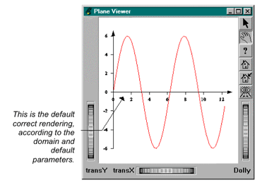
// tutorialGraph03.cxx
...
// Create the curve
PoCurve* myCurve = new PoCurve;
SbVec2f points[N_PT];
double ang;
int i;
for ( i = 0, ang = 0.; i < N_PT; i++, ang += 4. * PI / ( double )N_PT )
points[i].setValue( ang, 6. * sin( ang ) );
myCurve->point.setValues( 0, N_PT, points );
myCurve->set( "curvePointApp.material", "diffuseColor [1 0 0]" );
// Create simple automatic X and Y linear axis
// Do not forget to set the domain if you want
// default parameters to be correct...
PoLinearAxis* myXAxis = new PoLinearAxis;
myXAxis->start.setValue( SbVec3f( 0., 0., 0. ) );
myXAxis->end = 4.\* PI;
myXAxis->type = PoCartesianAxis::XY;
myXAxis->set( "appearance.material", "diffuseColor 0 0 0" );
PoLinearAxis* myYAxis = new PoLinearAxis;
myYAxis->start.setValue( SbVec3f( 0., -6., 0. ) );
myYAxis->end = 6.;
myYAxis->type = PoCartesianAxis::YX;
myYAxis->set( "appearance.material", "diffuseColor 0 0 0" );
// Create the root of the scene graph
SoSeparator* root = new SoSeparator;
root->ref();
// Define domain
#ifdef USE_PB
PbDomain myDom( 0., -6., 4.\* PI, 6. );
myXAxis->setDomain( &myDom );
myYAxis->setDomain( &myDom );
myCurve->setDomain( &myDom );
#else
PoDomain* myDom = new PoDomain;
myDom->min = SbVec3f( 0, -6, 0 );
myDom->max = SbVec3f( 4.\* PI, 6., 0 );
root->addChild( myDom );
#endif
root->addChild( myXAxis );
root->addChild( myYAxis );
root->addChild( myCurve );
SoXtPlaneViewer* viewer = new SoXtPlaneViewer( myWindow );
viewer->setSceneGraph( root );
viewer->setBackgroundColor( SbColor( 1., 1., 1. ) );
...
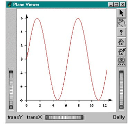 We perhaps want the axes to share the same origin, and not to cross each other. To make this, we simply have to change the origin of our X axis:
myXAxis->start.setValue( SbVec3f( 0., -6., 0. ) );
As we have already seen, you can customize these axes instead of using
default parameters and then get the following visualization using the following code. You
should notice that if tickSubDef field is set to PoAxis::PERIOD_MAIN_TICK
, it lets you choose if all the main ticks will be
annotated or only a subset of them by specifying a tickNumOrPeriod
. If tickSubDef is set to PoAxis::NUM_SUB_TICK, then the tickNumOrPeriod field is the number of sub-graduations between two main
graduations. Sub-graduations are never annotated. firstGrad and lastGrad fields allow you to control which first main tick and
which last main tick will be annotated if not all of them.
Example : Curve and axes with grid lines and sub-graduations
...
// Create simple automatic X and Y linear axis
// Do not forget to set the domain if you want
// default parameters to be correct...
PoLinearAxis* myXAxis = new PoLinearAxis;
myXAxis->start.setValue( SbVec3f( 0., -6., 0. ) );
myXAxis->end = 4. * PI;
myXAxis->step = 1.;
myXAxis->type = PoCartesianAxis::XY;
myXAxis->gridVisibility = PoAxis::VISIBILITY_ON;
myXAxis->gridLengthGradOtherSide = 12;
myXAxis->tickSubDef = PoAxis::PERIOD_MAIN_TICK;
myXAxis->setDomain( &myDom );
root->addChild( myXAxis );
PoLinearAxis* myYAxis = new PoLinearAxis;
myYAxis->start.setValue( SbVec3f( 0., -6., 0. ) );
myYAxis->end = 6.;
myYAxis->type = PoCartesianAxis::YX;
myYAxis->gridVisibility = PoAxis::VISIBILITY_ON;
myYAxis->gridLengthGradOtherSide = 4. * PI;
myYAxis->tickSubDef = PoAxis::NUM_SUB_TICK;
myYAxis->tickNumOrPeriod = 2;
myYAxis->setDomain( &myDom );
root->addChild( myYAxis );
...
 Notice that the grid lines are drawn on top of the curve. This is
because of the traversal order of the scene graph: the curve object is traversed (thus
drawn) before the axes. If you prefer to have the curve drawn on top of the grid, just add
the curve to the scene graph after adding the axes.
Using a Group of axes
Instead of creating two PoLinearAxis nodes we could have chosen to use a group of axes. GraphMaster provides five classes to deal directly with “boxes” of axes (2D and 3D axes):
- PoGroup2Axis
- PoGroup3Axis3
- PoGroup4Axis
- PoGroup6Axis3
- PoAutoCubeAxis The following program (located in $OIVHOME/src/MeshViz/Mentor) draws the same curve but this time using a PoGroup2Axis node. You will notice in this example that each individual axis may be customized in the same way as in the previous example. To do this, all you have to do is get the part corresponding to the axis in the PoGroup2Axis node kit using the SO_GET_PART Open Inventor macro and then edit whatever field you want on this specific axis:
Example : Using a group of axes 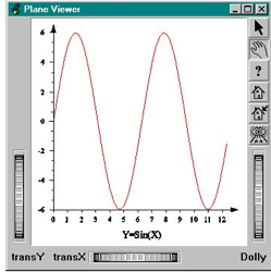
// tutorialGraph04.cxx
...
// Create the curve
PoCurve* myCurve = new PoCurve;
SbVec2f points[N_PT];
double ang;
int i;
for ( i = 0, ang = 0.; i < N_PT; i++, ang += 4. * PI / ( double )N_PT )
points[i].setValue( ang, 6. * sin( ang ) );
myCurve->point.setValues( 0, N_PT, points );
myCurve->set( "curvePointApp.material", "diffuseColor [1 0 0]" );
// Create a group of 2 axis and edit some fields of them
PoGroup2Axis* my2Axis = new PoGroup2Axis;
my2Axis->start.setValue( SbVec2f( 0., -6. ) );
my2Axis->end.setValue( SbVec2f( 4.\* PI, 6. ) );
my2Axis->xTitle = "Y=Sin(X)";
my2Axis->set( "appearance.material", "diffuseColor 0 0 0" );
PoLinearAxis* myXAxis = SO_GET_PART( my2Axis, "xAxis", PoLinearAxis );
PoLinearAxis* myYAxis = SO_GET_PART( my2Axis, "yAxis", PoLinearAxis );
myXAxis->step = 1.;
myYAxis->tickSubDef = PoAxis::NUM_SUB_TICK;
myYAxis->tickNumOrPeriod = 2;
// Create the root of the scene graph
SoSeparator* root = new SoSeparator;
root->ref();
#ifdef USE_PB
// Define domain
PbDomain myDom( 0., -6., 4.\* PI, 6. );
myCurve->setDomain( &myDom );
my2Axis->setDomain( &myDom );
#else
PoDomain* myDom = new PoDomain;
myDom->min = SbVec3f( 0, -6, 0 );
myDom->max = SbVec3f( 4.\* PI, 6., 0 );
root->addChild( myDom );
#endif
root->addChild( my2Axis );
root->addChild( myCurve );
SoXtPlaneViewer* viewer = new SoXtPlaneViewer( myWindow );
viewer->setSceneGraph( root );
viewer->setBackgroundColor( SbColor( 1., 1., 1. ) );
...
Several curves may also share the same axis system. The following example (located in $OIVHOME/src/MeshViz/Mentor) draws two curves sharing the same PoGroup2Axis node.
 Refer to the section called “Step 4: Multiple curves sharing one X axis and different Y axes”, if
you want to draw several curves that do not share the same axis system.
Example : Two curves sharing the same axes 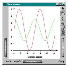
// tutorialGraph05.cxx
...
// Create the curves
double ang;
int i;
SbVec2f points1[N_PT];
PoCurve* myCurve1 = new PoCurve;
for ( i = 0, ang = 0.; i < N_PT; i++, ang += 4. * PI / ( double )N_PT )
points1[i].setValue( ang, 6. * sin( ang ) );
myCurve1->point.setValues( 0, N_PT, points1 );
myCurve1->set( "curvePointApp.material", "diffuseColor [1 0 0]" );
SbVec2f points2[N_PT];
PoCurve* myCurve2 = new PoCurve;
for ( i = 0, ang = 0.; i < N_PT; i++, ang += 4.\* PI / ( double )N_PT )
points2[i].setValue( ang, PI* cos( ang ) );
myCurve2->point.setValues( 0, N_PT, points2 );
myCurve2->set( "curvePointApp.material", "diffuseColor [0 1 0]" );
// Create a group of 2 axis and edit some fields of them
PoGroup2Axis* my2Axis = new PoGroup2Axis;
my2Axis->set( "appearance.material", "diffuseColor 0 0 0" );
my2Axis->start.setValue( SbVec2f( 0., -6. ) );
my2Axis->end.setValue( SbVec2f( 4.\* PI, 6. ) );
my2Axis->xTitle = "Multiple curves";
// Create the root of the scene graph
SoSeparator* root = new SoSeparator;
root->ref();
#ifdef USE_PB
// Define domain
PbDomain myDom( 0., -6., 4.\* PI, 6. );
myCurve1->setDomain( &myDom );
myCurve2->setDomain( &myDom );
my2Axis->setDomain( &myDom );
#else
PoDomain* myDom = new PoDomain;
myDom->min = SbVec3f( 0, -6, 0 );
myDom->max = SbVec3f( 4.\* PI, 6., 0 );
root->addChild( myDom );
#endif
root->addChild( myCurve1 );
root->addChild( myCurve2 );
root->addChild( my2Axis );
SoXtPlaneViewer* viewer = new SoXtPlaneViewer( myWindow );
viewer->setSceneGraph( root );
viewer->setBackgroundColor( SbColor( 1., 1., 1. ) );
...
Step 3: Animated data
You may want to display real-time data and then animate your curve. The following example (located in $OIVHOME/src/MeshViz/Mentor) shows this capability using an SoTimerSensor sensor from Open Inventor. At each time interval, a random number is generated and added to the curve. The X axis shows the step number and the Y axis the random value. The animation cycles through a maximum number of steps, N_PT. You will notice that the domain changes (no matter what kind of property classes are used) and then the display is updated automatically.
Example : An animated curve
// tutorialGraph06.cxx
...
#define N_PT 50
#define max( a, b ) (((a)>(b))?(a)/(b))
// Create the root of the scene graph
SoSeparator* root = new SoSeparator;
root->ref();
// Create the curve
myCurve = new PoCurve;
myCurve->point.setValues( 0, 0, points );
myCurve->setDomain( &myDom );
myCurve->set( "curvePointApp.material", "diffuseColor 1 0 0" );
root->addChild( myCurve );
// Create a group of 2 axis
my2Axis = new PoGroup2Axis;
my2Axis->xTitle = "Randomize";
my2Axis->set( "appearance.material", "diffuseColor 0 0 0" );
my2Axis->setDomain( &myDom );
root->addChild( my2Axis );
mySensor = new SoTimerSensor( newPointCB, NULL );
mySensor->setInterval( 10.0 );
mySensor->schedule();
...
}
static void
newPointCB( void*, SoSensor* )
{
int i;
float newy, ymax, x, y;
newy = 50. * rand() / RAND_MAX;
points[cur_n_pt].setValue( cur_n_pt, newy );
if ( cur_n_pt < N_PT - 1 )
cur_n_pt++;
else
{
cur_n_pt = 0;
myCurve->point.setNum( 0 );
return;
}
ymax = newy;
for ( i = 0; i < cur_n_pt; i++ )
{
points[i].getValue( x, y );
ymax = max( ymax, y );
}
myDom.setDomain( 0, 0, N_PT, ymax );
my2Axis->end.setValue( SbVec2f( N_PT, ymax ) );
myCurve->point.setValues( 0, cur_n_pt, points );
mySensor->schedule();
}
Step 4: Multiple curves sharing one X axis and different Y axes
The purpose of this section is to show the use of domain functionality when you want to draw multiple data sets which share the same X axis but have different Y domains. In the following example we are going to mix a bar chart representation with a curve representation. Each of the representations has a different Y domain but shares the same X domain.
Two things may be tricky when mixing axes like this. First, you must compute the Y translation for the second axis so that its origin will line up with the origin of the first Y axis. Then you must compute the X translation for the second Y axis so that it does not overlap the first one.
To compute the first translation, you must remember the domain transformation. Then you must compute the scale and/or the translation applied to the Y-axis coordinates because of this transformation. In our example we use the SCALE_X_FIXED transformation. This means that X will not be scaled and Y will be scaled by dx/dy (refer to the domain section in the What You Must Know about MeshViz XLM:). Our first axis domain is from -1 to 1 in Y and from 0 to 13 in X. All Y coordinates are thus scaled using a 2/13 factor. So the curve’s Y axis origin is (-1. * 13. / 2.) after the domain transformation. We can apply the same method to the bar chart’s Y axis. Its domain is from -10 to 20 for Y and from 0 to 13 for X. So the transformed Y origin is (-10. * 13. / 30.). We now have both Y coordinates in the same space where we will compute the translation to be applied. To compute the second translation, we will use the SoGetBoundingBoxAction action from Open Inventor. This action, when applied to the root of an axis system, will give you the real bounding box of this system, including ticks, arrows, and text strings. We can use the following skeleton if we want to build a visualization with multiple curves:
For all axis systems:
- Build the axis system.
- Add it to the root node of all axis systems .
- Compute the bounding box using the SoGetBoundingBoxAction action and apply it to the root node.
- Get the minimum x value of the bounding box.
- Use this value to translate the next axis system. This method allows you to build as many non-overlapping Y axes as you want. You can also, of course, use the same method if you want to have multiple X axes or multiple axes wherever you want. In fact, you can use the translation value to add a translation node to your scene graph or use this value as the X axis origin of your new axis (the next example, located in
$OIVHOME/src/MeshViz/Mentor, uses this second solution).
Example : A curve and a histogram sharing two different Y axes but the same X axis 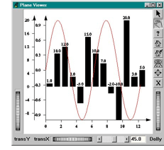
// tutorialGraph07.cxx
...
#define N_PT 50
#define PI 3.1315
// Create the curve
PoCurve* myCurve = new PoCurve;
SbVec2f points[N_PT];
double ang;
int i;
for ( i = 0, ang = 0.; i < N_PT; i++, ang += 4. * PI / ( double )N_PT )
points[i].setValue( ang, sin( ang ) );
myCurve->point.setValues( 0, N_PT, points );
myCurve->set( "curvePointApp.material", "diffuseColor [1 0 0]" );
// Create the root of the scene graph
SoSeparator* root = new SoSeparator;
root->ref();
// Domain of the curve
#ifdef USE_PB
PbDomain myCurveDom( 0., -1., 13., 1. );
myXAxis->setDomain( &myCurveDom );
myCurveYAxis->setDomain( &myCurveDom );
myCurve->setDomain( &myCurveDom );
#else
PoDomain* myCurveDom = new PoDomain;
myCurveDom->min = SbVec3f( 0, -1, 0 );
myCurveDom->max = SbVec3f( 13, 1, 0 );
root->addChild( myCurveDom );
#endif
root->addChild( myXAxis );
root->addChild( myCurveYAxis );
root->addChild( myCurve );
// We compute the bounding box of the first axis system
// So we will know how to translate the second Y axis
SoGetBoundingBoxAction myAction( SbViewportRegion( 1000, 1000 ) );
myAction.apply( root );
float xmin, ymin, zmin, xmax, ymax, zmax;
myAction.getBoundingBox().getBounds( xmin, ymin, zmin, xmax, ymax, zmax );
// Create the bar chart
PoSingleHistogram* myHist = new PoSingleHistogram;
myHist->start.setValue( 0., 0. );
myHist->end = 13.;
float values[13] = { 1., 10., 12., 3., -5., 15., 10., 7., -2., -10., 20., 3., 5. };
myHist->value.setValues( 0, 13, values );
myHist->set( "appearance.material", "diffuseColor 0 0 0" );
// Create Y axis for the bar chart
PoLinearAxis* myHistYAxis = new PoLinearAxis;
myHistYAxis->start.setValue( SbVec3f( xmin, -10., 0. ) );
myHistYAxis->set( "appearance.material", "diffuseColor 0 0 0" );
myHistYAxis->end = 20.;
myHistYAxis->type = PoCartesianAxis::YX;
// Domain of the histogram
#ifdef USE_PB
PbDomain myHistDom( 0., -10, 13., 20. );
myHistYAxis->setDomain( &myHistDom );
myHist->setDomain( &myHistDom );
#else
PoDomain* myHistDom = new PoDomain;
myHistDom->min = SbVec3f( 0, -10, 0 );
myHistDom->max = SbVec3f( 13, 20, 0 );
root->addChild( myHistDom );
#endif
// Now we have to align horizontally the two Y axis
SoTranslation* myTrans = new SoTranslation;
float trans;
trans = ( -130. / 30. ) - ( -13. / 2. );
myTrans->translation.setValue( 0., -trans, 0. );
// Complete the scene graph (The curve will be drawn after bar chart.
// The translation should only apply to the bar chart and its Y axis
root->addChild( myTrans );
root->addChild( myHistYAxis );
root->addChild( myHist );
SoXtPlaneViewer* viewer = new SoXtPlaneViewer( myWindow );
viewer->setSceneGraph( root );
viewer->setBackgroundColor( SbColor( 1., 1., 1. ) );
...
Step 5: Adding a key to a visualization
If you draw business graphs you may want to identify the different parts of your visualization. In this section we are going to look at the PoItemLegend node derived from PoLegend class. All key nodes derived from this class will be illustrated in the 3DdataMaster part of this manual. When you draw curves with GraphMaster, you may use a line representation or draw it using markers for instance. The PoItemLegend node allows you to annotate your visualization with legends corresponding to the different types of visualization you use in your display. Items in the legend include an optional text string, an optional colored box, an optional set of markers, and an optional line. You can change the appearance of each of these parts. The items may be arranged in one or several columns. Depending on the size of the bounding box of all items (which you specify when you create the legend node), GraphMaster will compute the text height, the box sizes, the number of markers to be drawn, and/or the length of the lines. You cannot control these attributes, but you can adjust margins around these items and the aspect ratio of the filled boxes. Here are some examples of legends you can create:
The following example (located in $OIVHOME/src/MeshViz/Mentor) draws a set of curves and then adds a legend to the display in order to identify these curves.
Example : Adding a legend to your set of curves 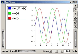
// tutorialGraph08.cxx
...
// Create the legend
PoItemLegend* myLegend = new PoItemLegend;
myLegend->start.setValue( -10., 7. );
myLegend->end.setValue( -3, 2 );
myLegend->item.set1Value( 0, "sin(x)" );
myLegend->item.set1Value( 1, "cos(x)" );
myLegend->item.set1Value( 2, "sin(x)\*cos(x)" );
SbColor colors[3] = { SbColor( 1., 0., 0. ), SbColor( 0., 1., 0. ), SbColor( 0., 0., 1. ) };
myLegend->boxColor.setValues( 0, 3, colors );
myLegend->set( "backgroundApp.material", "diffuseColor 1 1 1" );
myLegend->set( "backgroundBorderApp.material", "diffuseColor 0 0 0" );
myLegend->set( "boxBorderApp.material", "diffuseColor 0 0 0" );
myLegend->set( "valueTextApp.material", "diffuseColor 0 0 0" );
#define PI 3.1415
#define N_PT 50
// Create X axis
PoLinearAxis* myXAxis = new PoLinearAxis;
myXAxis->set( "appearance.material", "diffuseColor 0 0 0" );
myXAxis->start.setValue( SbVec3f( 0., -1., 0. ) );
myXAxis->end = 4.\* PI;
myXAxis->type = PoCartesianAxis::XY;
// Create Y axis
PoLinearAxis* myYAxis = new PoLinearAxis;
myYAxis->set( "appearance.material", "diffuseColor 0 0 0" );
myYAxis->start.setValue( SbVec3f( 0., -1., 0. ) );
myYAxis->end = 1.;
myYAxis->type = PoCartesianAxis::YX;
// Create the curves
double ang;
int i;
PoCurve* myCurve1 = new PoCurve;
SbVec2f points1[N_PT];
for ( i = 0, ang = 0.; i < N_PT; i++, ang += 4.\* PI / ( double )N_PT )
points1[i].setValue( ang, sin( ang ) );
myCurve1->point.setValues( 0, N_PT, points1 );
myCurve1->set( "curvePointApp.material", "diffuseColor [1 0 0]" );
PoCurve* myCurve2 = new PoCurve;
SbVec2f points2[N_PT];
for ( i = 0, ang = 0.; i < N_PT; i++, ang += 4.\* PI / ( double )N_PT )
points2[i].setValue( ang, cos( ang ) );
myCurve2->point.setValues( 0, N_PT, points2 );
myCurve2->set( "curvePointApp.material", "diffuseColor [0 1 0]" );
PoCurve* myCurve3 = new PoCurve;
SbVec2f points3[N_PT];
for ( i = 0, ang = 0.; i < N_PT; i++, ang += 4.\* PI / ( double )N_PT )
points3[i].setValue( ang, sin( ang ) * cos( ang ) );
myCurve3->point.setValues( 0, N_PT, points3 );
myCurve3->set( "curvePointApp.material", "diffuseColor [0 0 1]" );
// Create the root of the scene graph
SoAnnotation* root = new SoAnnotation;
root->ref();
root->addChild( myLegend );
#ifdef USE_PB
// Define domain
PbDomain myDom( 0., -1., 4.\* PI, 1. );
myXAxis->setDomain( &myDom );
myYAxis->setDomain( &myDom );
myCurve1->setDomain( &myDom );
myCurve2->setDomain( &myDom );
myCurve3->setDomain( &myDom );
#else
PoDomain* myDom = new PoDomain;
myDom->min = SbVec3f( 0, -1, 0 );
myDom->max = SbVec3f( 4.\* PI, 1., 0 );
root->addChild( myDom );
#endif
root->addChild( myXAxis );
root->addChild( myYAxis );
root->addChild( myCurve1 );
root->addChild( myCurve2 );
root->addChild( myCurve3 );
SoXtPlaneViewer* viewer = new SoXtPlaneViewer( myWindow );
viewer->setSceneGraph( root );
viewer->setBackgroundColor( SbColor( 1., 1., 1. ) );
...
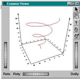
You may have noticed in the previous example that the legend is transformed in the same way as the curves during camera manipulation. If the plane viewer is replaced by an Examiner Viewer and if we change the 3D view, we will then get a display like this.
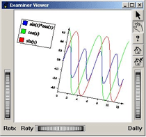 Since we did not define any camera in the previous examples, the plane or examiner viewers add their own at the top of our scene graph to manipulate the scene.
To avoid any view transformation inheritance in the legend node, all we
have to do is add our own camera node to the scene graph, between the legend node and the
axis and curves nodes. The viewers will then use this camera and any changes made to this
camera will affect the axes and the curves, but not our legend node.In the following code, you will notice the changes for the start and end fields of the
legend node. As the legend will not be affected by the viewer camera nor by the camera we
have included in the scene graph, the default view will be used to render this node, and the
default space for this view is [-1,1]x[-1,1].
Furthermore, MeshViz supplies classes to manage multiple views. These
classes are PoBaseView
,PoView
, and PoSceneView (see the Reference Manual for more information).
Example : Adding a legend that is independent of the viewing 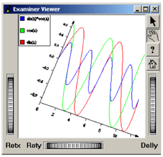
...
// Create the legend
PoItemLegend* myLegend = new PoItemLegend;
myLegend->start.setValue( -1., 1. );
myLegend->end.setValue( -.5, .5 );
myLegend->item.set1Value( 0, "sin(x)" );
...
root->addChild( myLegend );
SoPerspectiveCamera* myCamera = new SoPerspectiveCamera;
root->addChild( myCamera );
// Define domain of curve and its axis.
#define PI 3.1415
PbDomain myDom( 0., -1., 4.\* PI, 1. );
...
SoXtExaminerViewer* viewer = new SoXtExaminerViewer( myWindow );
myCamera->viewAll( root, viewer->getViewportRegion() );
viewer->setSceneGraph( root );
...
Step 6: An example of a 3D visualization
 All that we have seen concerning 2D applies in the same way to 3D. Instead of a 2D domain, we will deal with a 3D domain. The following example (located in $OIVHOME/src/MeshViz/Mentor) builds a 3D curve and displays it with its 3D axis system. Here we will use the PoGroup6Axis node. As with PoGroup2Axis which we have already used, the SO_GET_PART Open Inventor macro may be used to retrieve each axis of the node kit. You can then customize each axis if the default representation does not suit your needs.
Example : Representing a 3D curve
// tutorialGraph09.cxx
...
#define N_PT 50
#define PI 3.1415
// Create the curve
double ang,
radius;
int i;
PoCurve3* myCurve = new PoCurve3;
SbVec3f points[N_PT];
ang = 0;
radius = 0.;
for ( i = 0; i < N_PT; i++, ang += 6. * PI / ( double )N_PT, radius += 10. / ( double )N_PT )
points[i].setValue( radius* cos( ang ), radius* sin( ang ), 2. * radius );
myCurve->point.setValues( 0, N_PT, points );
myCurve->set( "curvePointApp.material", "diffuseColor [1 0 0]" );
myCurve->set( "curvePointApp.drawStyle", "linewidth 3." );
// Create the group of axis
PoGroup6Axis3* my6Axis = new PoGroup6Axis3;
my6Axis->set( "appearance.material", "diffuseColor 0 0 0" );
my6Axis->start.setValue( -10., -10., 0. );
my6Axis->end.setValue( 10., 10., 20. );
// Create the root of the scene graph
SoSeparator* root = new SoSeparator;
root->ref();
// Define domain of curve and its axis.
#ifdef USE_PB
PbDomain myDom( -10., -10., 0., 10., 10., 20. );
myCurve->setDomain( &myDom );
my6Axis->setDomain( &myDom );
#else
PoDomain* myDom = new PoDomain;
myDom->min = SbVec3f( -10., -10., 0. );
myDom->max = SbVec3f( 10., 10., 20. );
root->addChild( myDom );
#endif root->addChild( myCurve );
root->addChild( my6Axis );
SoXtExaminerViewer* viewer = new SoXtExaminerViewer( myWindow );
viewer->setSceneGraph( root );
viewer->setBackgroundColor( SbColor( 1., 1., 1. ) );
...
Enhanced Business Graphics Nodes
Introduction
GraphMaster supplies a package of more than fifty classes specifically targeting high level 3D business visualization. Easy to use, this package brings the power of 3D graphics to your business data. These representations include: high level display of curves as tubes, ribbons or “wall curves” with variable thickness and material mapping; customized 3D histograms; 3D pie charts with beveled edges; and an amazing variety of other chart types.
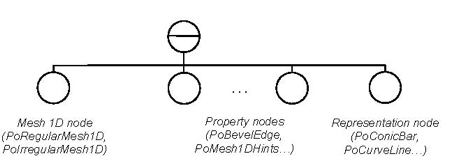
GraphMaster has three categories of nodes:
- Data storage nodes: These are one-dimensional meshes (meshes inherited from the abstract class PbMesh1D ) used for charting representations. Data storage is independent of the 3D representation.
- Property nodes: These nodes allow the user to specify the appearance of the representations nodes.
- Representation nodes: These are node kits, all inherited from PoChart , to draw tubes, ribbons,… A classical scene graph using these nodes looks like the following:
Enhanced business graphics property nodes
The mesh classes usually used for 3DdataMaster representations have been extended to one-dimensional meshes in order to store data for charting representations.
"Important"
Property nodes specify the appearance of the representation classes. Only classes inherited from PoChart take into account these properties.
Enhanced business graphics node classes
To draw cylindrical bars

To draw bars where each bar is defined by a scene graph.

To draw bars where each bar is defined by a line.

To draw bars where each bar is defined by the current profile (see PoProfile nodes).

To build a 2D curve line. The thickness of the curve can be constant or may depend on a value-set of the current 1D mesh.

To draw a 3D filled curve.

To build a 2D ribbon curve.

To build a 2D tube curve. The profile of the tube is given by the current profile (see PoProfile nodes).

A generalized scatter representation is a marker field representation where each marker is defined by a scene graph.

A scatter representation is a bitmap marker field (the SoMarkerSet shape is used for this representation).
To build a 3D pie chart. The height of each slice can be constant or may depend on the value-set of the current 1D mesh.

To draw a label field. Figure 2.47. Enhanced business graphics node classes
An example
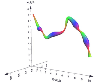 The following example (located in $OIVHOME/src/MeshViz/Mentor) displays a tube curve with an elliptic profile curve where the thickness and the color is variable for each vertex of the curve.
Example : A tube curve
// tutorialGraph10.cxx
...
#define NP 14
float x[NP] = { 0.5, 1.5, 1.8, 2.4, 3.2, 4.5, 6.3, 6.9, 8.0, 8.5, 9.0, 9.5, 9.8, 10 };
float y[NP] = { 9.0, 7.0, 6.5, 6.0, 5.0, 5.5, 6.0, 7.7, 6.8, 6.0, 5.5, 4.5, 3.5, 2.5 };
float size[NP] = { 1, 3, 5, 1, 3, 5, 1, 3, 5, 1, 3, 5, 1, 3 };
SbColor colorListD[3] = { SbColor( 1, 0, 0 ), SbColor( 0, 1, 0 ), SbColor( 0, 0, 1 ) };
// Domain of the representation from [0,0,-1] to [10,1O,1]
PoDomain* myDomain = new PoDomain;
myDomain->min.setValue( 0., 0., -1 );
myDomain->max.setValue( 10., 10., 1 );
// Font use for axis
PoMiscTextAttr* myTextAttr = new PoMiscTextAttr;
myTextAttr->fontName = "Courier";
SoSeparator* root = new SoSeparator;
// Define the irregular 1D mesh for the geometry of the tube curve.
PoIrregularMesh1D* mesh1D = new PoIrregularMesh1D;
mesh1D->setGeometry( NP, x ); // Abscissas of the tube.
mesh1D->addValuesSet( 0, y ); // Ordinates of the tube.
mesh1D->addValuesSet( 1, size ); // Values-set for the variable
// sizes of the tube.
// The tube will be smoothed.
PoMesh1DHints* mesh1DHints = new PoMesh1DHints;
mesh1DHints->geomInterpretation = PoMesh1DHints::SMOOTH;
// Material use by the tube.
SoMaterial* mat = new SoMaterial;
mat->diffuseColor.setValues( 0, 3, colorListD );
// Defined the elliptic profile of the tube.
PoEllipticProfile* profile = new PoEllipticProfile;
profile->xRadius = 0.15;
profile->yRadius = 0.025;
// Define the tube curve representation.
PoTube* tube = new PoTube;
tube->material.setValue( mat );
tube->colorBinding = PoTube::PER_VERTEX;
tube->thicknessFactor = 0.5;
tube->thicknessIndex = 1;
// Defines the three axis.
PoGroup2Axis* g2Axis = new PoGroup2Axis( SbVec2f( 0., 0. ), SbVec2f( 10., 10. ), PoGroup2Axis::LINEAR, PoGroup2Axis::LINEAR, "X-Axis", "Y-Axis" );
PoLinearAxis* zAxis = new PoLinearAxis( SbVec3f( 0, 0, -1 ), 1, PoLinearAxis::ZY );
// Builds the scene graph.
root->ref();
root->addChild( mesh1D );
root->addChild( myDomain );
root->addChild( myTextAttr );
root->addChild( mesh1DHints );
root->addChild( profile );
root->addChild( tube );
root->addChild( zAxis );
root->addChild( g2Axis );
// Builds the examiner viewer.
SoXtExaminerViewer* viewer = new SoXtExaminerViewer( myWindow );
viewer->setSceneGraph( root );
viewer->setTitle( "Tube" );
...
Frequently asked questions about GraphMaster
Why is the text on my axis very tiny?
The size of the text on your axis is expressed as a percentage of the domain. This is also true for certain other axis attributes and other representations. Either you have forgotten to define a domain (PoDomain), or you have not defined it correctly.
Why does MeshViz use a domain (PoDomain) instead of a classic scale
(SoScale)?
There are several reasons for the existence of the domain.
First imagine that you have a curve that ranges from 0 to 1 along the x-axis and from 0 to 1000 in the y-axis. You want to represent this curve and also the axis system associated with it.
If you don’t use a transformation, the resulting display will not be legible because the y-axis is very large compared to the x-axis. Intuitively you will want to scale the y-axis relative to the x-axis (or vice versa) in order to obtain something legible. If you do this using an SoScale, it will work for the curve representation (PoCurve) but you will have some problems with the axis representation (PoLinearAxis). Specifically, you will note that the graduation labels as well as the arrow at the end of the axis will appear very flattened along the direction of the Y-axis. So, applying a simple scale transformation is not the correct way to achieve a good result because some parts of your representation need to be uniformly scaled but not others.
The property node PoDomain addresses these kinds of problems.
Second, many fields of MeshViz nodekits are expressed in the space defined by the current domain. The chapter on Domains of the MeshViz User’s Guide provides additional details about the use of domains.
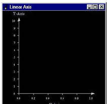
How can I generate an axis representation that is not square?
Generally, you define the domain values as the bounding box of your data and you obtain a square representation.
For instance, if you want to have an X-axis from 0 to 1 and a Y-axis from 0 to 10, you set the domain (PoDomain) fields to: min (0,0,0) and max (1,10,1).
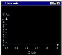
 Now, if you want to obtain an X-axis which is double the size of the Y-axis, you must define a domain which has double the size of the Y-data – that is, min (0,0,0) and max (1,20,1) – and you obtain the following:
 In the first case (square representation), the scale applied by the PoDomain to the axis is the following:
min and max are the fields of the PoDomain node.
dx = max[0] - min[0]
dy = max[1] - min[1]
dz = max[2] - min[2]
Sx = 1: the end coordinate of the X-Axis is 1.
Sy = dx/dy = 1 / 10 = 0.1 -> the top coordinate of the Y-Axis is 10 x 0.1 = 1.
Sz = dx/dz = 1 / 1 = 1
In the second case (rectangular representation), the scale applied by the PoDomain to the axis is the following:
Sx = 1 : the end coordinate of the X-Axis is 1.
Sy = dx/dy = 1 / 20 = 0.05 -> the top coordinate of the Y-Axis is 10 x 0.05 = 0.5
Sz = dx/dz = 1 / 1 = 1
How can I preserve the aspect ratio of my data while using a
domain?
As described in the previous question, defining the domain values as the bounding box of your data gives a square representation. However if you absolutely need to preserve the aspect ratio of your data, you can use the PoDomain::setValues() method with the last argument set to MIN_BOUNDING_CUBE.
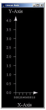
For instance, if you want to have an X-axis from 0 to 1 and an Y-axis from 0 to 5, and preserve the original (1 to 5) aspect ratio:
myDomain->setValues(SbVec3f(0,0,0), SbVec3f (1,5,1), PoDomain::MIN_BOUNDING_CUBE);
 ##### How can I use Open Inventor shapes (SoCube/CoCone,…) and MeshViz shapes when I use a PoDomain?
All MeshViz shapes automatically insert in their catalog kit (part named domainTransform) a transformation which corresponds to the domain, so these shapes are automatically transformed. For Open Inventor shapes, you must add this transformation to the scene graph manually just before the shape to be transformed. To get the transformation that should be applied, call the PoDomain::getMatrixTransform() method which returns an SoMatrixTransform.
Why do SoFont nodes inserted just before my axis seems to be
ignored?
All MeshViz representations ignore the node SoFont for selecting the font name and size. Instead the property node PoMiscTextAttr is used for this purpose.
How can I change the numeric format of the graduations of my
axis/legend/pie chart/histograms/…?
The property node PoNumericDisplayFormat manages the format of all numeric values displayed by MeshViz. Insert this node with the requested format in the scene graph just before the representation to be configured.